Speeding up spatial operations in R
I am a big fan of R’s spatial libraries, especially sf for vector data and terra for raster data. In fact, I could write a great essay about the reasons why you should use R for your spatial analysis (it makes things easily replicable, it integrates well with other languages you might use in a project, it’s free, etc.), but I’ll leave that subtweet of ArcGIS for another day.
For all of their magical features, I do sometimes find myself confronting non-trivial memory/timing barriers when using the R spatial libraries locally for my projects. This is particularly true when—as is often the case for me—I need to do things involving geometric binary predicates with many different geometries.
One way that I’ve been getting around this recently is through batch processing. Making use of a pretty simple helper function from the sf package, sf::st_make_grid(), I can easily break up my spatial operations into more memory-manageable chunks.
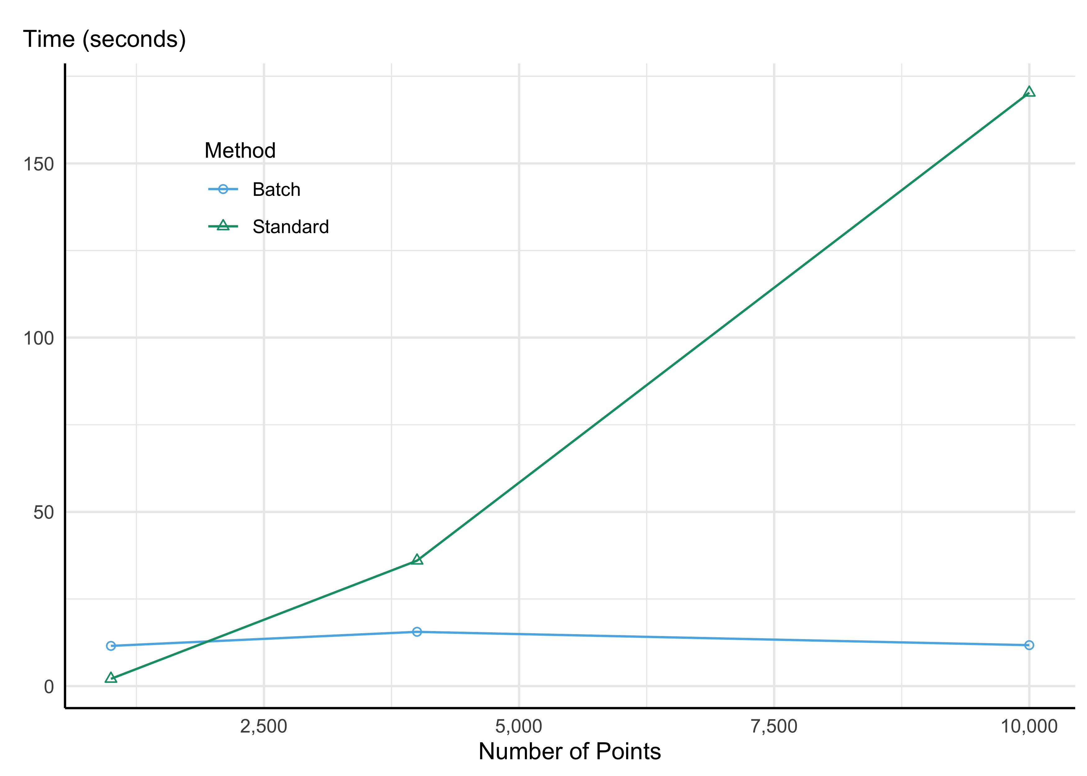
Say, for instance, I have a bunch of points for each of which I want to identify points falling a certain distance, say a mile. The sf package has a nice function for this: sf::st_is_within_distance(); however, if I have a lot of points using this function in the “standard” way would involve a non-trivial number of distance calculations (e.g., 10,000 points would mean 100,000,000 distance calculations!!). And most of those calculations are useless: I can easily rule out certain point-pairs as being outside of the target distance of say 1 mile.
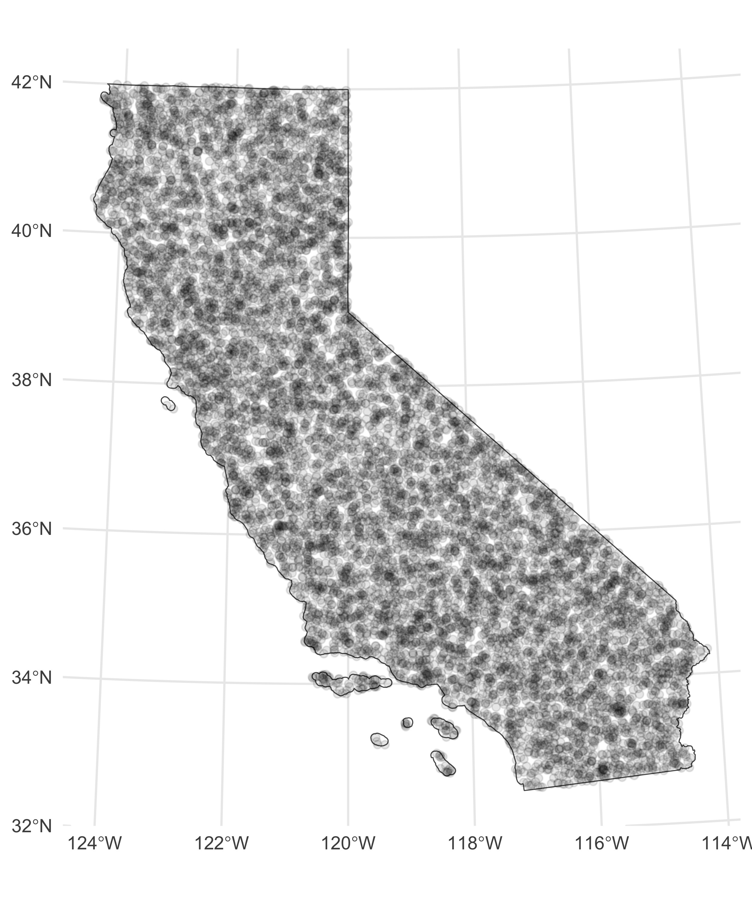
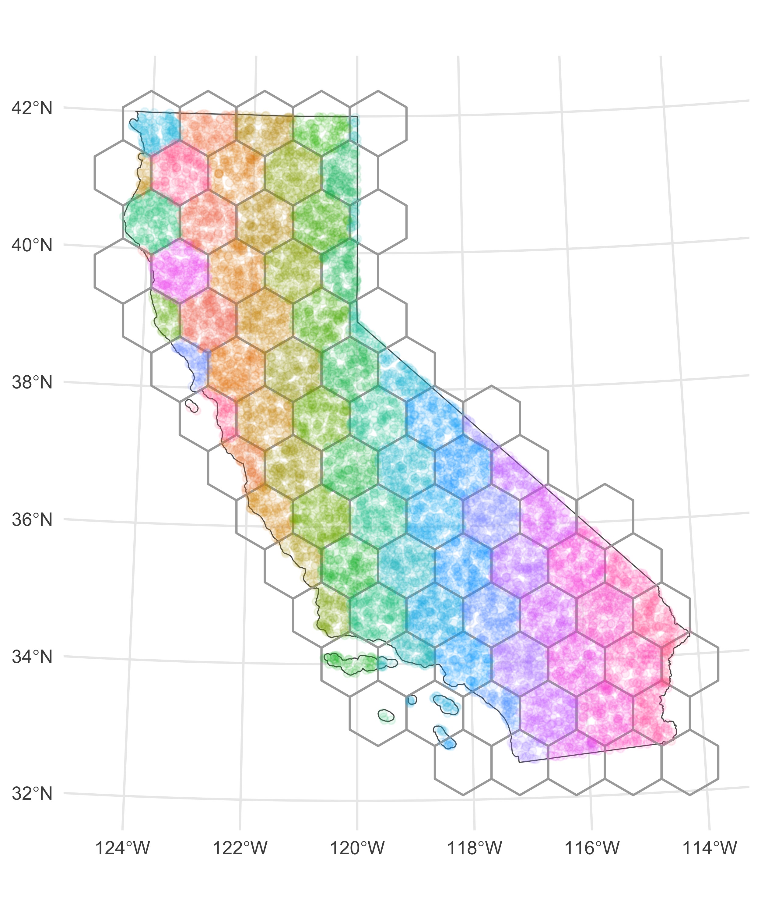
Let’s make this example a bit more concrete. Say we have 10,000 points within the state of California chosen at random. I can use the function sf::st_make_grid() to break up the spatial extent of this area into a specified number of grids (actually hexagons, but you can also do square grids — the hexagons fit spatial data a bit better). Once I’ve done that, I can make use of the sf::st_join() function to assign each of my points to a given grid, then I can loop over each grid when doing my intensive spatial operations.
1
2
3
4
5
6
7
8
9
10
11
12
13
14
 # Load dependencies:
pacman::p_load(sf, tigris)

# Download California county shapefiles:
ca.counties <- tigris::counties(state = "CA") %>%
	st_transform(., crs = st_crs(3310))

# Sample points:
sample.points <- st_sample(ca.counties, 10000) %>%
	st_sf

# Create 10x10 grid:
ca.grid <- st_make_grid(ca.state, n=c(10,10), square = F) %>%
	st_sf
The square=F argument makes a grid of hexagons with the same extent of the California county polygons. Now if you’re paying close attention, you might worry about how points at the edges of each grid are handled with this approach. Surely there might be some points falling within the target distance for points on the boundary of a given grid that are in other grids. To get around this, we can actually buffer the grid polygons we’ve created by the target distance—here I’m using a mile—and then do the st_join() with our points:
1
2
3
4
5
 # Create one-mile buffer around CA grid:
ca.grid.buffer <- st_buffer(ca.grid, dist.within)

# Intersect buffered grid with sampled points:
sample.points <- st_join(sample.points, ca.grid.buffer)
The side-by-side images below show the initial problem and the resulting batch assignments.


1
2
3
4
 # Standard approach:
standard <- microbenchmark(
	st_is_within_distance(sample.points, dist = dist.within, remove_self = T)
)
1
2
3
4
 # Batch process:
batch <- microbenchmark(
	sample.points[ , .(res = list(st_is_within_distance(.SD[['geometry']], dist = dist.within, remove_self = T))), by = id]
)
